Top 50 Data Science Interview Questions in 2026 What Each Tests and How to Answer Strongly
DS-INTERVIEW System and DEPTH-PLUS-EXAMPLE formula for all 50 Data Science interview questions in India 2026 seven domains, GenAI section, and 14-day sprint.
Mrityunjay Pandey
· 13 July 2026 ·17 min read
Share:
Contents
Direct Answer:
Data Science technical interviews in India in 2026 test seven distinct knowledge domains statistics, machine learning concepts, Python and coding, model evaluation, feature engineering, generative AI, and business communication and the 10 questions in this guide that most decisively determine an offer are the ones where the answer quality reveals whether you understand the concepts or have memorised the definitions, because that distinction is exactly what the interviewer is trying to determine.
This is not a Q&A list to memorise. It is a preparation guide that uses the DEPTH-PLUS-EXAMPLE Answer Formula define, explain the reasoning, give a specific example to show what strong answers look like across all 50 questions, organised by the seven interview stages they come from.
The DS-INTERVIEW Preparation System
A seven-domain wheel or hub visual showing the DS-INTERVIEW Preparation System — seven sections labelled: Statistics (with icons for normal distribution, p-value, hypothesis test), Machine Learning (with icons for decision tree, neural network, ensemble), Python and Data Handling (Pandas, NumPy, Scikit-learn icons), Model Evaluation (confusion matrix, ROC curve icons), Feature Engineering (encoding, scaling, selection icons), Generative AI and LLMs (GPT, RAG, embedding icons), and Business Communication (project walkthrough, stakeholder icon). The centre of the wheel shows "Data Science Technical Interview India 2026." Each domain segment shows the number of questions in this guide (e.g., Statistics: Q11–Q18). A callout shows: "Assess your domain strength before starting your sprint."
(See the framework visual above)
The DS-INTERVIEW Preparation System maps your preparation across seven stages. Before using this guide, assess which stages are your strongest and which need the most work. The 10 most decisive questions cut across multiple stages understanding which stage each comes from tells you where to invest more preparation time.
The 10 Most Decisive Questions Full Depth Coverage
Question 1 — Explain the Bias-Variance Trade-Off
What it tests: This is the fundamental test of whether you understand how machine learning models generalise. It separates candidates who understand why models fail from those who only know how to run them.
Weak answer: “Bias is when the model is too simple and variance is when the model is too complex.”
Strong answer: “The bias-variance trade-off describes the two primary sources of prediction error in a machine learning model. Bias is error from incorrect assumptions in the learning algorithm a high-bias model pays too little attention to the training data, producing predictions that are consistently off in the same direction. This is underfitting. Variance is error from sensitivity to small fluctuations in the training set a high-variance model pays too much attention to the training data, producing predictions that are highly accurate on training data but highly inaccurate on new data. This is overfitting.
The trade-off exists because reducing bias typically increases variance and vice versa. A very simple model (high bias, low variance) will consistently make the same prediction regardless of the input — a linear model applied to a non-linear problem. A very complex model (low bias, high variance) will fit every quirk of the training data including noise — a decision tree with unlimited depth. The goal of model selection and regularisation is to find the complexity level where the total prediction error (bias squared plus variance) is minimised on new data.
In my project, I observed this when comparing a logistic regression model (high bias — underfitting the relationship between features and the target) with a random forest with no depth restriction (high variance — achieving 99% training accuracy but only 72% test accuracy). I resolved it by tuning the random forest’s max_depth and min_samples_leaf hyperparameters, producing a test accuracy of 84% with substantially reduced variance.”
Question 2 — What Is Overfitting and How Do You Fix It?
What it tests: Practical model debugging knowledge and the ability to connect symptoms to solutions.
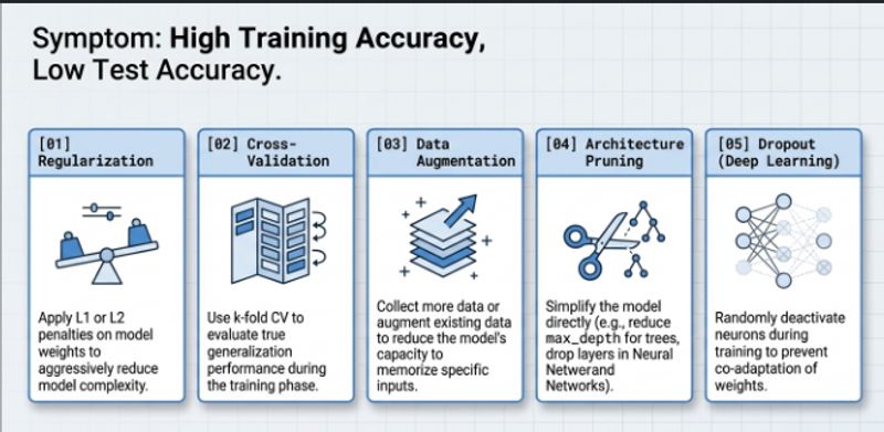
Strong answer structure: Define overfitting (high training accuracy, low test accuracy, the model has learned noise in the training data rather than the underlying pattern). Explain why it happens (model too complex for the amount of training data). List specific techniques with brief reasoning: (1) Regularisation — L1 or L2 penalties on model weights reduce complexity. (2) Cross-validation — use k-fold CV to evaluate true generalisation performance and catch overfitting during training. (3) More data — if the dataset is small, augmentation or additional collection reduces the model’s ability to memorise specific examples. (4) Simpler model — reduce max_depth for trees, reduce layers for neural networks. (5) Dropout — for neural networks, randomly deactivating neurons during training prevents co-adaptation. Give one specific example from your project.
Question 3 — Explain Precision vs Recall — When Do You Use Each?
What it tests: Metric selection judgment under real-world constraints — the most commonly misunderstood pair of evaluation metrics.
Weak answer: “Precision is true positives divided by all predicted positives. Recall is true positives divided by all actual positives.”
Strong answer: “Precision answers: of everything I predicted as positive, how many were actually positive? Recall answers: of everything that was actually positive, how many did I correctly identify? The choice between optimising for precision versus recall depends on the cost of each type of error.
When false positives are expensive, optimise for precision. In spam filtering, a false positive means a legitimate email is marked as spam — the user misses an important email. A high-precision spam filter flags fewer legitimate emails as spam, even if it misses some actual spam. When false negatives are expensive, optimise for recall. In cancer screening, a false negative means a patient with cancer receives a negative result — the disease goes untreated. A high-recall cancer screen catches more actual cancer cases, even if it flags some healthy patients for further investigation.
F1 score is the harmonic mean of precision and recall, used when you need a single metric that balances both. In my fraud detection project, I optimised for recall — missing a fraudulent transaction (false negative) was more costly than flagging a legitimate transaction for review (false positive).”
Question 4 — What Is the Difference Between L1 and L2 Regularisation?
What it tests: Mathematical understanding of how regularisation works, not just that it exists.
Strong answer: “Both L1 and L2 regularisation reduce overfitting by adding a penalty term to the loss function that discourages large model weights. L1 regularisation (Lasso) adds the absolute value of the weights to the loss — this penalty can drive individual weights all the way to zero, effectively performing feature selection by removing the contribution of less important features entirely. L2 regularisation (Ridge) adds the square of the weights — this distributes the penalty more evenly, shrinking all weights toward zero but rarely eliminating them completely.
The mathematical reason for this difference: the L1 penalty has a constant gradient regardless of the weight magnitude, so it pushes weights toward zero equally aggressively until they reach zero. The L2 penalty has a gradient proportional to the weight magnitude, so as a weight approaches zero, the push toward zero weakens — it shrinks but rarely reaches exactly zero.
The practical implication: use L1 when you believe many features are irrelevant and want the model to select the most important ones automatically. Use L2 when you believe most features contribute meaningfully and want to reduce their influence without eliminating any. Elastic Net combines both penalties, which is useful when you have many correlated features.”
Question 5 — Explain Your Project End to End
This is covered in the Project Walkthrough section later in this guide. The structure is identical to the one described in but adapted to the Data Science context: problem statement, data source and preparation steps, feature engineering decisions, model selection and reasoning, evaluation metrics and results, challenges encountered and resolved, and what you would improve.
Question 6 — What Is a P-Value and What Does It Tell You?
What it tests: Statistical reasoning. P-values are the most commonly misunderstood concept in statistics and the question that most reliably separates candidates with genuine statistical understanding from those with surface familiarity.
Weak answer: “A p-value less than 0.05 means the result is statistically significant.”
Strong answer: “A p-value is the probability of observing the test result (or a more extreme result) assuming that the null hypothesis is true. If the p-value is very small — conventionally below 0.05 — it means that the data we observed would be very unlikely if the null hypothesis were true. This gives us statistical evidence to reject the null hypothesis in favour of the alternative.
What a p-value does NOT tell you: it does not tell you the probability that the null hypothesis is true. It does not tell you the size or practical importance of the effect. A study with a very large sample can produce a statistically significant p-value for an effect so small that it has no practical relevance. This is the distinction between statistical significance and practical significance.
For example, if I run an A/B test on two landing page variants and get a p-value of 0.03, I can say: if the two variants were identical, we would observe a difference this large or larger only 3% of the time by chance. This is evidence the difference is real. But if the actual conversion rate difference is 0.1% — from 10.0% to 10.1% — the practical significance may not justify the implementation cost, even though the statistical significance is confirmed.”
Question 7 — How Would You Handle Imbalanced Classes in a Classification Problem?
What it tests: Practical problem-solving beyond textbook knowledge.
Strong answer: “Class imbalance occurs when one class has significantly more samples than another for example, fraud detection where 99% of transactions are legitimate and 1% are fraudulent. Training a standard classifier on this data produces a model that predicts the majority class for everything and still achieves 99% accuracy — which is useless for the minority class we actually care about.
The standard approaches and when to use each: (1) Resampling — oversampling the minority class (SMOTE: Synthetic Minority Oversampling Technique generates synthetic minority class samples) or undersampling the majority class. SMOTE is generally preferred because it generates new samples rather than duplicating existing ones. (2) Class weights — most sklearn models accept a class_weight parameter that penalises misclassification of the minority class more heavily during training, without changing the training data. (3) Threshold adjustment — instead of using the default 0.5 probability threshold for classification, adjust the threshold to optimise for recall on the minority class. (4) Ensemble methods — algorithms like BalancedRandomForest and EasyEnsemble are specifically designed for imbalanced datasets.
In my project, I used SMOTE combined with class weights and evaluated on precision, recall, and F1 for the minority class rather than overall accuracy — because overall accuracy is a misleading metric for imbalanced problems.”
Question 8 — What Is Gradient Descent and How Does It Work?
What it tests: Mathematical intuition about how machine learning models learn — essential for understanding why training sometimes fails.
Strong answer: “Gradient descent is the optimisation algorithm that most machine learning models use to find the parameter values that minimise the loss function. The intuition: imagine you are standing on a hilly landscape in fog, trying to find the lowest point. You cannot see the whole landscape, so you take a step in the downward direction from where you are standing — the direction of steepest descent — and repeat. Eventually you reach a local minimum.
Mathematically, gradient descent computes the partial derivative (gradient) of the loss function with respect to each model parameter, then updates each parameter in the direction opposite to the gradient, scaled by the learning rate. The learning rate controls step size: too large and the algorithm overshoots the minimum and may diverge; too small and convergence is very slow.
The three variants: Batch gradient descent uses the full training dataset to compute each gradient — accurate but slow for large datasets. Stochastic gradient descent (SGD) uses one randomly selected sample per update — fast but noisy. Mini-batch gradient descent uses a small random subset per update — the balance used in practice, including in all deep learning frameworks.
In my neural network project, I used Adam optimiser — an adaptive learning rate variant of gradient descent that adjusts the learning rate for each parameter individually based on recent gradient history — which converged faster than vanilla SGD for my classification task.”
Question 9 — What Is the Difference Between Bagging and Boosting?
What it tests: Ensemble method understanding at the reasoning level, not the definition level.
Strong answer: “Both bagging and boosting are ensemble methods that combine multiple weak models into a stronger model, but they do so through fundamentally different mechanisms.
Bagging (Bootstrap Aggregating) trains multiple models in parallel on different random subsets of the training data (with replacement) and combines their predictions by averaging (regression) or voting (classification). The key effect is reducing variance: each model sees slightly different data, so their errors are not correlated, and averaging their predictions smooths out individual errors. Random Forest is bagging applied to decision trees.
Boosting trains models sequentially, where each model focuses on correcting the errors of the previous models. The training data is reweighted after each model so that misclassified examples receive more weight in the next model’s training. The final prediction is a weighted combination of all models, with more accurate models receiving higher weight. The key effect is reducing bias: each sequential model reduces the error that remained after the previous models. XGBoost, LightGBM, and AdaBoost are boosting algorithms.
The practical choice: use bagging (Random Forest) when you are worried about overfitting it averages out high-variance individual trees. Use boosting (XGBoost, LightGBM) when you want maximum predictive accuracy and have sufficient data it systematically reduces error but can overfit if not regularised. In competitions and production classification tasks with structured data, boosting algorithms typically outperform bagging.”
Question 10 — What Is an LLM and How Does RAG Improve It?
What it tests: Current AI knowledge expected in Data Science interviews in 2026 given the integration of GenAI into the data science workflow.
Strong answer: “A Large Language Model is a neural network trained on enormous volumes of text to predict the next token in a sequence. Through this training on diverse text data, LLMs develop the ability to generate coherent, contextually appropriate text, answer questions, write code, summarise documents, and perform a wide range of language tasks. The intelligence emerges from the statistical patterns learned during training rather than from explicit rules.
The key limitation for enterprise applications: an LLM’s knowledge is frozen at its training cutoff. It cannot access information that postdates its training, and it has no knowledge of private organisational data. When asked about things outside its training distribution, it may hallucinate — generating confident-sounding but incorrect information.
RAG (Retrieval-Augmented Generation) addresses this by connecting the LLM to an external knowledge source at inference time. When a query arrives, a retrieval system first finds relevant documents from the knowledge base (using vector similarity search on text embeddings), then provides those documents as context to the LLM alongside the query. The LLM generates a response grounded in the retrieved documents rather than purely in its training knowledge. The result is more accurate, more current, and more attributable responses for domain-specific queries.
In my RAG project, I built a document QA system over a company’s internal policy documents using LangChain, Chroma as the vector store, and the OpenAI API as the generation layer. The system answered HR policy questions accurately by grounding responses in the retrieved policy document sections.”
Category 1 — Statistics and Probability (Questions 11 to 18)
Q11: What is the Central Limit Theorem? Define it (the distribution of sample means approaches normal as sample size grows, regardless of the population distribution), explain why it matters (underpins hypothesis testing and confidence intervals), give an example (sampling customer purchase amounts — individual amounts are skewed, but mean purchase amounts across samples are normally distributed).
Q12: What is Bayes’ Theorem and when is it used? P(A|B) = P(B|A) × P(A) / P(B). Explain the update of prior belief based on new evidence. Application: spam filter updating the probability that an email is spam based on the presence of specific words.
Q13: Explain the difference between correlation and causation. Correlation measures the strength of the linear relationship between two variables. Causation means one variable directly causes changes in the other. Classic example: ice cream sales and drowning rates are correlated (both increase in summer) but neither causes the other — temperature is the confounding variable.
Q14: What is a confidence interval? A range of values that contains the true parameter with a specified probability (e.g., 95% CI means if we repeated the experiment many times, 95% of the constructed intervals would contain the true parameter). Common misconception: it does not mean there is a 95% probability the true value is in this specific interval.
Q15: What are Type I and Type II errors? Type I (false positive): rejecting a true null hypothesis. Type II (false negative): failing to reject a false null hypothesis. Relate to precision/recall: Type I error rate is 1 — precision; Type II error rate is 1 — recall. Significance level α controls Type I error.
Q16: What is the difference between parametric and non-parametric tests? Parametric tests assume the data follows a specific distribution (usually normal). Non-parametric tests make no distributional assumptions. Use non-parametric tests when the data is ordinal, when the sample is small, or when normality cannot be assumed.
Q17: What is A/B testing and what statistical test would you use? A/B testing compares two variants to determine which performs better. For conversion rates (binary outcomes), use a chi-squared test or z-test for proportions. For continuous metrics (revenue, time on site), use a t-test after checking normality assumptions.
Q18: What is the difference between covariance and correlation? Covariance measures how two variables change together but is not standardised — its magnitude depends on the scale of the variables. Correlation standardises covariance by the product of standard deviations, producing a value between -1 and 1. Correlation is covariance divided by the product of standard deviations.
Category 2 — Machine Learning Concepts (Questions 19 to 30)
Q19: What is the difference between supervised, unsupervised, and reinforcement learning? Supervised: labelled data, predict output from input. Unsupervised: unlabelled data, find structure (clustering, dimensionality reduction). Reinforcement: agent learns through rewards and penalties from environment interactions. Examples: supervised — email classification; unsupervised — customer segmentation; reinforcement — game-playing agents.
Q20: What is the difference between classification and regression? Classification predicts a discrete categorical label. Regression predicts a continuous numeric value. Same algorithms often have both variants (decision trees, neural networks). Logistic regression despite its name is a classification algorithm.
Q21: Explain decision trees and their advantages and disadvantages. Decision trees split data recursively by the feature that produces the greatest information gain (or Gini reduction). Advantages: interpretable, handles non-linear relationships, no feature scaling required. Disadvantages: highly sensitive to training data (high variance), prone to overfitting with deep trees. Solved with ensemble methods (Random Forest, Gradient Boosting).
Q22: What is K-means clustering and what are its limitations? K-means partitions data into K clusters by iteratively assigning each point to the nearest centroid and updating centroids to the mean of their cluster. Limitations: requires specifying K in advance, assumes spherical clusters of similar size, sensitive to outliers, may converge to local minima depending on initialisation.
Q23: What is dimensionality reduction and why is it used? Reducing the number of features while preserving as much information as possible. Reasons: reduce computational cost, mitigate the curse of dimensionality, remove correlated features, enable visualisation. Techniques: PCA (linear, maximises variance), t-SNE and UMAP (non-linear, for visualisation), autoencoders (deep learning).
Q24: What is Principal Component Analysis (PCA)? PCA finds the directions (principal components) in feature space that account for the most variance in the data, and projects the data onto the top K components. Each component is a linear combination of original features. PCA is unsupervised — it does not consider the target variable. The key concept is that components are orthogonal (uncorrelated).
Q25: What is the difference between K-Nearest Neighbours and K-means? KNN is a supervised classification algorithm — it predicts the label of a new point based on the labels of its K nearest neighbours in training data. K-means is an unsupervised clustering algorithm — it finds K cluster centres without any labels. The K in both algorithms means something different.
Q26: Explain Support Vector Machines. SVMs find the hyperplane that maximises the margin between classes — the distance from the hyperplane to the nearest training points (support vectors) of each class. The kernel trick allows SVMs to find non-linear decision boundaries by implicitly mapping features into higher-dimensional space where a linear boundary exists.
Q27: What is a neural network and what is the role of activation functions? Neural networks are layers of interconnected nodes (neurons) that transform input data through weighted connections. Each neuron computes a weighted sum of its inputs and applies an activation function. Activation functions introduce non-linearity — without them, a neural network is equivalent to a single linear transformation regardless of depth. Common activations: ReLU (avoids vanishing gradient, default for hidden layers), Sigmoid (outputs probability, used in binary classification output), Softmax (outputs class probabilities, used in multi-class classification).
Q28: What is the vanishing gradient problem? During backpropagation in deep neural networks, gradients are multiplied repeatedly as they flow backward through layers. If each multiplication reduces the gradient magnitude (as with sigmoid and tanh activations), gradients in early layers become extremely small — these layers learn very slowly or not at all. Solutions: ReLU activations, batch normalisation, residual connections (skip connections in ResNets).
Q29: What is transfer learning? Reusing a model trained on one task as the starting point for a model on a different but related task. Rather than training from random weights, start with weights learned on large data (e.g., ImageNet for vision, Wikipedia + books for language) and fine-tune on task-specific data. Effective when labelled data is limited for the target task.
Q30: What is the difference between generative and discriminative models? Discriminative models learn the boundary between classes — P(Y|X), the probability of a label given features. Examples: logistic regression, SVM, neural network classifiers. Generative models learn the distribution of data — P(X|Y) and P(Y) — and can generate new data samples. Examples: Naive Bayes, GANs, VAEs. Generative AI models (GPT, Claude) are generative models trained on text.
Category 3 — Python and Data Handling (Questions 31 to 38)
Q31: How do you handle missing values in Pandas? Detect with df.isnull().sum(). Options: (1) Drop rows/columns with df.dropna(). (2) Fill with mean/median/mode using df.fillna(). (3) Forward/backward fill for time series. (4) Predict missing values using model imputation (KNNImputer, IterativeImputer from sklearn). Choice depends on missing data mechanism (MCAR, MAR, MNAR) and proportion of missing data.
Q32: What is the difference between apply, map, and applymap in Pandas? map applies a function element-wise to a Series. apply applies a function along a row or column axis of a DataFrame, or element-wise to a Series. applymap (now map in newer Pandas) applies a function element-wise to every element of a DataFrame. Use apply for column/row transformations, map for Series value mapping.
Q33: How do you merge two DataFrames in Pandas? pd.merge(df1, df2, on=’column’, how=’inner/outer/left/right’). Equivalent to SQL JOIN operations. inner: only matching rows. outer: all rows from both, NaN for non-matches. left: all rows from left DataFrame. right: all rows from right DataFrame.
Q34: What is the difference between loc and iloc in Pandas? loc selects by label (column name or row index label). iloc selects by integer position. When the DataFrame index is integer-based and sequential, they produce the same result — but when the index is non-sequential or string-based, they behave differently. Safe practice: always use loc for label-based selection and iloc for position-based selection.
Q35: How do you detect and handle outliers? Detection: IQR method (values below Q1–1.5×IQR or above Q3 + 1.5×IQR), Z-score (values beyond 3 standard deviations), visualisation (box plots, scatter plots). Handling: (1) Remove if data entry error. (2) Cap/floor (Winsorisation) if genuine extreme values. (3) Treat as separate segment. (4) Use robust algorithms (tree-based models are naturally outlier-resistant).
Q36: Write a Python function to calculate the moving average of a list. Tests basic Python proficiency. Solution: def moving_average(data, window): return [sum(data[i:i+window])/window for i in range(len(data)-window+1)]. Alternative using Pandas: pd.Series(data).rolling(window).mean().
Q37: What is the difference between deep copy and shallow copy in Python? Shallow copy creates a new object that references the same nested objects. Deep copy creates a new object with completely independent copies of all nested objects. Relevant in data pipelines where modifying a copy should not affect the original — use copy.deepcopy() for nested data structures.
Q38: How do you work with JSON data in Python and convert it to a DataFrame? import json; data = json.loads(json_string) or with open(‘file.json’) as f: data = json.load(f). Convert to DataFrame: pd.json_normalize(data) for nested JSON flattening, or pd.DataFrame(data) for flat JSON arrays.
Category 4 — Model Evaluation and Selection (Questions 39 to 46)
Q39: What is a confusion matrix? A 2×2 matrix (for binary classification) showing True Positives, True Negatives, False Positives, and False Negatives. The foundation for computing precision, recall, F1, and accuracy. Always look at the confusion matrix first — overall accuracy alone is misleading for imbalanced datasets.
Q40: What is the ROC-AUC score? ROC (Receiver Operating Characteristic) curve plots True Positive Rate vs False Positive Rate at various classification thresholds. AUC (Area Under the Curve) summarises the entire ROC curve as a single number between 0 and 1. AUC of 0.5 means the model is no better than random. AUC of 1.0 means perfect discrimination. Use AUC for comparing models, not for setting the classification threshold.
Q41: When would you use RMSE vs MAE for regression evaluation? RMSE (Root Mean Square Error) penalises large errors more heavily due to squaring — use when large errors are particularly undesirable. MAE (Mean Absolute Error) treats all errors equally more robust to outliers. If your data has outliers and you do not want the metric to be dominated by them, prefer MAE.
Q42: What is k-fold cross-validation? Splitting the training data into k equal folds, training on k-1 folds, and validating on the remaining fold, repeated k times so each fold serves as the validation set once. The k model performance scores are averaged for a more robust estimate of generalisation performance than a single train/test split. Stratified k-fold maintains class proportions in each fold essential for imbalanced datasets.
Q43: How do you choose between models? Factors: performance on appropriate metrics for the task, computational cost (training and inference time), interpretability requirements (regulatory contexts often require explainable models), data size (deep learning requires large data), deployment constraints. Use cross-validation to compare, not test set performance the test set is for final evaluation only.
Q44: What is data leakage and how do you prevent it? Data leakage occurs when information from outside the training period is included in the model’s features, producing optimistic performance estimates that do not generalise. Examples: using future data to predict past events, including the target variable’s derived features, scaling the entire dataset before splitting into train/test. Prevention: always split data before any transformation, use pipelines to apply transformations within cross-validation folds.
Q45: What is the difference between validation set and test set? Validation set is used during model development for hyperparameter tuning and model selection — it is seen many times. Test set is used only once, after all development is complete, for the final unbiased estimate of model performance. Using the test set for model selection constitutes data leakage on the test set.
Q46: How do you handle multi-class classification? One-vs-Rest (OvR): train K binary classifiers, each distinguishing one class from all others. One-vs-One (OvO): train K(K-1)/2 binary classifiers, one for each pair of classes. Softmax directly produces probabilities across all classes. For evaluation, extend precision/recall/F1 to multi-class using macro (unweighted average), weighted (class-frequency weighted), or micro (aggregate across all classes) averaging.
Category 5 — Feature Engineering (Questions 47 to 51)
Q47: What is feature selection and what methods are available? Removing irrelevant or redundant features to reduce dimensionality, improve model performance, and reduce training time. Filter methods: statistical tests (chi-squared, ANOVA, correlation) applied before modelling. Wrapper methods: sequential forward/backward selection using model performance as the criterion. Embedded methods: regularisation (L1) or tree-based feature importance that select features as part of model training.
Q48: How do you encode categorical variables? Nominal (no order): one-hot encoding (creates binary columns for each category), or target encoding (replace category with mean target value). Ordinal (ordered): label encoding (assign integers preserving order). High-cardinality features: target encoding or embeddings. One-hot encoding increases dimensionality — be aware of multicollinearity.
Q49: What is the difference between normalisation and standardisation? Normalisation (Min-Max Scaling): scales values to [0,1] range. Standardisation (Z-score normalisation): scales values to have mean 0 and standard deviation 1. Use normalisation when the distribution is not Gaussian and when you need values in a bounded range. Use standardisation when the data follows (approximately) a Gaussian distribution. Tree-based models (decision trees, random forests) do not require scaling — distances are not used. Linear models, SVM, and neural networks benefit from scaling.
Q50: How do you create new features from existing ones? Domain-driven feature creation: date features (day of week, month, is_weekend from datetime), interaction features (product of two correlated features), ratio features (revenue per customer, profit margin). Polynomial features for capturing non-linear relationships. Text features using TF-IDF or embeddings. Lag features for time series. Signal: domain knowledge about what relationships are meaningful is more valuable than automated feature generation.
The GenAI and LLM Questions (Questions 41 to 45 in a 2026 Interview)
These five questions have become standard in Data Science interviews since 2024 and are now expected at the fresher level.
What is fine-tuning an LLM vs using RAG? Fine-tuning trains the model on additional data, updating its weights expensive, requires significant data, changes the model permanently. RAG provides external context at inference time without changing the model cheaper, more flexible, better for frequently changing data.
What are embeddings? Numerical vector representations of text (or other data) that capture semantic meaning. Similar concepts have similar vectors (small cosine distance). Used in semantic search, recommendation systems, and RAG pipelines.
What is prompt engineering? Designing the text instructions provided to an LLM to produce more accurate, structured, or appropriate outputs. Techniques: few-shot examples, chain-of-thought reasoning, role specification, output format specification.
What is hallucination in LLMs and how do you mitigate it? Hallucination is when an LLM generates confident, plausible-sounding but factually incorrect information. Mitigations: RAG (ground responses in retrieved sources), temperature reduction (less randomness in generation), output verification pipelines, explicitly instructing the model to say “I don’t know” when uncertain.
How would you evaluate an LLM-based application? Traditional ML metrics do not apply directly. Use: RAGAS (RAG-specific evaluation framework), human evaluation, LLM-as-judge (using a separate LLM to evaluate response quality), retrieval metrics (precision@k, recall@k), and task-specific metrics (BLEU/ROUGE for text generation, exact match for factual QA).
The Contrarian Truth About Data Science Interview Preparation
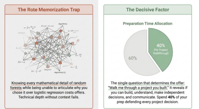
A visual illustrating the contrarian insight — showing two candidate profiles side by side. Profile A (Algorithm Depth): knows every mathematical detail of random forests, gradient descent derivation, and kernel trick — labelled "Strong on paper, average in interview." Profile B (Project Ownership): can explain every feature engineering decision, articulate why Random Forest was chosen over logistic regression for their specific dataset, describe the specific challenge of class imbalance and how SMOTE was applied — labelled "Average algorithm depth, strong interview performance." A callout shows the contrarian truth: "Project walkthrough preparation (40%+ of prep time) produces higher offer probability than additional algorithm coverage.
Here is the insight that most Data Science interview preparation guides avoid: the question that most consistently determines an offer in a Data Science fresher interview is not about algorithm mathematics or Python syntax — it is “walk me through a project you built” because this one question reveals every other thing the interviewer needs to know: whether you have built anything, whether you understand what you built, whether you made independent decisions, and whether you can communicate technical work clearly.
The common assumption is that Data Science interview success comes from knowing more algorithms more depth on gradient descent, more understanding of the mathematics of SVM, more coverage of rare evaluation metrics. This preparation produces candidates who are impressive on paper and average in interviews, because the technical depth questions are only part of what determines an offer.
The project walkthrough is where genuine preparation produces the largest return: knowing every mathematical detail of random forests while being unable to articulate why you chose random forest over logistic regression for your specific project, what the most important feature in your model was and why it makes business sense, and what you would do differently if you rebuilt the project these are the gaps that cost offers. Spend at least 40% of your preparation time on your project and your ability to defend every decision in it.
Tactical Section: The 14-Day Data Science Interview Sprint
Days 1 to 2 — Project audit. Without notes, explain your project end-to-end including: data source and cleaning steps, feature engineering decisions and reasoning, model selection and why (what alternatives you considered and rejected), evaluation metrics and results, production considerations. Record yourself. Identify every hesitation point.
Days 3 to 5 — The 10 decisive questions. Prepare full DEPTH-PLUS-EXAMPLE answers for all 10 most decisive questions from this guide. Practice each out loud until the answer flows without visible effort.
Days 6 to 8 — Category coverage. Work through each of the seven DS-INTERVIEW categories. For each question you cannot answer fully, write the Layer 2 (reasoning) and Layer 3 (example) components and practice them out loud.
Days 9 to 11 — Python and coding practice. Complete five coding exercises in a blank environment without reference: a Pandas data cleaning pipeline, a group-by aggregation query, a custom function using list comprehensions, a matplotlib visualisation, and a Scikit-learn pipeline. Write out loud.
Days 12 to 13 — Full mock interview. Conduct a complete mock technical interview covering statistics questions, ML concept questions, coding, project walkthrough, and one GenAI question. Record it. Review for hesitation and clarity gaps.
Day 14 — Light review and confidence. Review your project’s design decisions and key metrics. Confirm your GitHub repositories are accessible. Prepare two genuine questions to ask the interviewer.
Data Science interviews test seven domains: statistics, ML concepts, Python, model evaluation, feature engineering, GenAI/LLMs, and business communication. All seven must be covered in preparation.
The 10 most decisive questions are those where answer quality most strongly predicts offer decisions — bias-variance trade-off, overfitting, precision/recall, L1/L2 regularisation, project walkthrough, p-values, imbalanced classes, gradient descent, bagging vs boosting, and LLMs/RAG.
The DEPTH-PLUS-EXAMPLE Answer Formula applies to every Data Science question: define the concept, explain the reasoning behind the design, give a specific example from your project or a well-known application.
GenAI questions (LLMs, RAG, embeddings, fine-tuning, hallucination) are now standard at the Data Science fresher interview level in India in 2026 and must be prepared explicitly.
The contrarian truth: the project walkthrough is the single most decisive element of a Data Science interview — more preparation time on defending every decision in your project produces higher returns than additional algorithm coverage.
The 14-day sprint provides a milestone-based preparation plan calibrated to the actual interview format rather than a passive review of all 50 questions.
Download the Free Data Science Interview Preparation Guide all 50 questions with DEPTH-PLUS-EXAMPLE answer frameworks, the 14-day sprint schedule, the project walkthrough script template, and the DS-INTERVIEW Preparation System category checklist used by Itdaksh Education’s Data Science students before placement drives.
Itdaksh Education 201 Ganesh Tower, Opposite Thane Railway Station, Thane West. ISO 9001:2015 and MSME Certified. Data Science with AI, Data Analytics, Python Full Stack. Rated 4.9/5 on Google.
#Data Science interview questions India 2026
#DS-INTERVIEW Preparation System
# DEPTH-PLUS-EXAMPLE Data Science
#machine learning interview India
#bias variance trade-off interview
#LLM RAG interview Data Science
#Itdaksh Education Data Science
#Mrityunjay Pandey
#14-day Data Science sprint
#Data Science project walkthrough

 Chat to Support